Deconstructing Grokking: How a Tiny Transformer Learns Modular Arithmetic
A foray into mechanistic interpretability

Why
Modern AI models are often considered black boxes — they magically find patterns and output the right answer. The internal mechanisms and processes that ChatGPT undergoes with every prompt are extremely difficult for humans to understand.
This has worrying implications for the future: both governments and companies seem far more invested in AI’s ability to generate profit than in our ability to understand what a model does under the hood.
While researching this issue, I came across articles about “mechanistic interpretability,” where researchers use different tools and techniques to reverse-engineer a model’s internal components — like its activations and weights — into algorithms and logical flows that humans can understand.
Mechanistic interpretability holds strong potential — in my opinion, more so than regulation, as governments are reluctant and move far too slow — to be the reins for AI in an age where we outsource an increasing number of our tasks and responsibilities to models that we don’t fully understand.
What
To learn more about the field, I decided to do my own mechanistic interpretability experiment based off Neel Nanda’s “A Mechanistic Interpretability Analysis of Grokking.”
What is “grokking?” No, it’s not related to Twitter’s AI model. Instead, grokking is a phenomenon where a model achieves near 100% training accuracy while having extremely low test accuracy (a clear sign that the model has overfitted the training data) for thousands of “epochs” (passes of the dataset through the model) before the test accuracy suddenly spikes to 100% and the model generalizes perfectly.
In essence, the model goes from “memorizing” the training data to “understanding” the pattern.
To understand the mechanics of this phase transition, I replicated the setup from Power et al. (2022) using a 1-layer transformer trained on modular addition. This post details the experimental design, architectural constraints, and specific mechanistic interpretability techniques (PCA, FFT, probing, and patching) used to reverse-engineer the model’s algorithm.
The code, graphs, and results for this experiment can be found on my GitHub.
EXPERIMENTAL DESIGN
The Task
Given inputs a and b, predict c such that c = a + b (mod p). a and b are natural numbers from [0, 112].
I fixed p = 113 for all experiments. I chose 113 for two reasons:
It’s prime. Prime numbers make it difficult for the model to find an illegitimate solution (no zero divisors, multiplicative inverses for all non-zero values). This makes it much more likely that the model will learn the clock-like algorithm needed for modular addition.
It’s large but not too large. The model has 114 tokens (integers 0-112 and a “=” token represented by 113). This is small enough, being less than the number of neurons/size of the embedding space (d_model = 128). It’s also enough large enough that the model cannot simply create a lookup table for each pair of a and b as it would require significant memory.
Model Architecture
I used a standard decoder-only transformer with strict constraints to ensure interpretability:
Layers: 1 (multiple layers substantially increase complexity)
Model dimension (d_model): 128 (represents the problem well without being overly large)
Attention heads: 4 (standard practice and can represent multiple frequencies, leaves every head sizable at 32)
MLP dimension (d_mlp): 512 (standard 4x expansion for transformers)
Context length: 3 (input is (a, b, 113), 113 represents “=”)
Activation function: ReLU (removes noise, ideal for experiment)
I disabled regularization and normalization to remove noise from the experiment.
Training Hyperparameters
Optimizer: AdamW (standard)
Learning rate: 0.001 (standard)
Weight decay: 1.0 (encourages grokking by penalizing large weights, model solutions in favor of simpler algorithms)
Batch size: Entire training dataset (small enough to do full batch)
Epochs: 10,000 (high to allow time to grok)
Variables
Any good experiment needs variables, controls, and multiple trials. After noticing that the initialization of the model and the split of the dataset created high variance, I chose three variables: training fraction (the fraction of the dataset the model is trained on), split seed (a seed that determines what data becomes training data), and model seed (a seed that initializes the model’s random weights).
I started with a training fraction of 30%, as higher training fractions would likely cause the model to generalize too quickly. The split seed and model seed were arbitrarily initialized at 0.
RUNNING EXPERIMENTS
To compare results across different split seeds, model seeds, and training fractions, I ran 29 different experiments: 20 where the training fraction and split seed were held constant while the model seed varied from zero to 19, five where only the split seed varied from one to five, and four where only the training fraction changed from 0.4 to 0.7. It is worth noting that I originally ran experiments with the training fraction initialized at 0.2 and changing from 0.3 to 0.6, but all of the models trained on only 20% of the dataset failed to grok. There are two possible explanations for this: either earlier findings are correct that grokking requires specific hyperparameters to occur, or the models happened to have bad weight initializations and would eventually grok after the 10,000 epoch limit. Future experiments should raise the epoch limit to test this theory.
Seven out of the 29 experiments failed to grok, with six of such experiments being where only the model seed varied and one being where only the split seed varied. Given that these seeds were arbitrarily selected and merely concern the random generation of the model weights and training data splits respectively, there is no reason to believe that the seven models failed to grok for any reason but random chance.
For the rest of the models, the results were largely what we would expect.
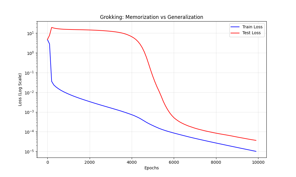
As the example above shows, the models’ train losses (weighted function of the difference between the actual answer and the model’s answer) quickly dropped to 0.001, but the test losses stayed around .15-.17. At some point from epochs 5000-9000, test loss would suddenly drop.
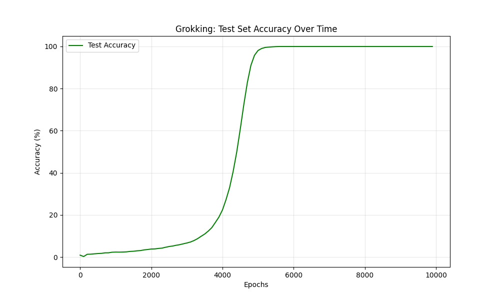
Interestingly, the models’ test accuracies did not remain completely flat before grokking. Instead, they increased to 17-20%. If the model was merely memorizing the training data, we would expect the test accuracy to stay low, but the slow increase in test accuracies suggests that the models may have already learned the algorithm for modular addition before grokking.


I consider this hypothesis as I use various mechanistic interpretability techniques to analyze the models.
Among the 29 experiments, there were some interesting cases where the results did not fully align with my expectations:
I recorded the model’s state and epoch pre-training, mid-training but before grokking (arbitrarily defined as the last hundredth epoch before test accuracy increased past 15%), and post-training. Surprisingly, models that crossed the 15% test accuracy threshold at a similar epoch had large variance in how long they took to grok (defined as the last hundredth epoch before test accuracy increased past 99%).
One example of this is experiments 1 and 2 (model seed 0 and model seed 1), where the models mid-training epochs were 3899 and 3799 respectfully. Experiment 1 grokked at epoch 9000 while experiment 2 grokked at epoch 5100.
This variance is likely due to the fact that although the models reach 15% test accuracy around the same time, different weight initializations mean that stochastic gradient descent may “luck” into finding the right algorithm quicker for one model than another.
The increases in training fraction caused the models to grok quicker and quicker. While the model with model and split seeds of 0 and a training fraction of 0.3 took 9000 epochs to grok, the models with the same seeds but training fractions of 0.4, 0.5, 0.6, and 0.7 grokked at 2500, 800, 600, and 300 epochs, respectively. This suggests that models are able to more easily generalize the algorithm when more of the data is present.
MODEL ANALYSIS
The following techniques can be applied to models to gain a better confidence and understanding of the mechanisms underlying a model’s performance.
Principal Component Analysis (PCA)
I used principal component analysis (PCA) to find the two most important components (dimensions) in the embedding space. PCA reduces noise and the number of dimensions from 128 to two, so it is extremely useful in increasing the interpretability of the model.
I performed PCA on models pre-training, mid-training but before grokking, and post-training.


The results revealed what I expected. Pre-training, the random embeddings generated at model initialization form a disordered cloud with no discernible structure. Post-training, the embeddings form a clearly distinguishable circle. Points that are mathematically adjacent modulo 113, e.g., 5 and 6, are also adjacent points on the circles. This shows a strong, albeit qualitative, signal that the model has discovered the clock-like nature of modular addition.
Discrete Fourier Transform (DFT)
To find the specific frequencies of the clock, I computed the discrete Fourier transform (DFT) of each neuron across the token index dimension. Given the results of the PCA, there is reason to believe that the model may be using trigonometric wave functions (sine and cosine) to represent the clockwork of modular addition.
In modular arithmetic, the most natural way to add two numbers is to treat them as rotations. If the model represents a number x using sine and cosine waves of a specific frequency ω: vx = [cos(ωx), sin(ωx)], then addition becomes a simple linear rotation operation (using standard trigonometric identities like sin(a + b) = sin a cos b + cos a sin b).
I applied DFT to test whether the model had learned trigonometric identities. Once again, I graphed the DFT of the pre-training, mid-training, and post-training models.


In the pre-training spectrum, the energy of the neurons is distributed roughly uniformly across all frequencies, with no prominent peaks. This is as expected, as the weights are all randomly initialized.
The mid-training spectrum is interesting — among the noise, there are faint striped bands for certain frequencies. This suggests that the model has already learned some of the trigonometric wave functions, lending more evidence for our earlier hypothesis.
The post-training spectrum shows that energy has concentrated in specific frequency components, often related to each other (multiples of 7, multiples of other frequencies represented.)
A quick calculation shows that the energy in these 4-6 target frequencies can exceed 80% of the total, with the remaining 20% distributed across all other frequencies.
The results of the DFT lends strong evidence to the hypothesis that the model has learned trigonometric identities to solve modular addition.
Ablation
I decided to use ablation, where I would remove frequencies/components of the model to test the effect on its performance, to verify whether the important frequencies shown by the DFT were the main frequencies responsible for the model’s perfect test accuracy.
I originally planned to identify the top three target frequencies (k = 12, 14, 19) and identify random frequencies with approximately the same energy. I would then ablate each set of frequencies and measure the drop in performance, using the random frequencies to act as a baseline to confirm that changes in performance were not purely attributable to the removal of 80% energy, but rather the removal of the specific three target frequencies.
However, since the target frequencies constituted ~80% of the total energy, finding random frequencies that summed to approximately the same total was mathematically impossible unless we included target frequencies in the list of random frequencies to pick from (in which case it would become difficult to determine what caused changes in performance).
Since energy-based frequency matching wouldn’t work, I chose to instead ablate three random frequencies. While this strategy was less ideal, it still provided a baseline comparison that could help determine whether changes in performance could be attributed to a mere ablation of any three frequencies or if the frequencies identified in the DFT were unique.
The results were as expected — ablating target frequencies caused performance to drop from 99% accuracy to approximately 1%, essentially returning the model to its pre-training state, while ablating random frequencies caused performance to dip by only one or two percentage points. This indicates that the frequencies related to the trigonometric identities are responsible for the grokking phenomenon.
Linear Probing
For the following probing and patching analysis, I selected six representative models:
Early1, Early2: Grokked by epoch 2,500.
Mid1, Mid2: Grokked by epoch 4,000-4,500.
Late1, Late2: Grokked after epoch 6,000.
This allowed me to test whether the speed of grokking affected the mechanism the model developed (and vice versa).
By training a linear probe — a ridge regression model — to predict cos(kx) and sin(kx) from the residual stream activations (after the model’s attention and MLP but just before its output), we can determine how well the trigonometric features generalize to the model’s “final answer” activations.
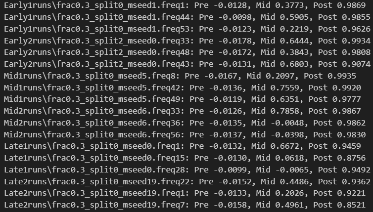
The resulting R^2 scores reinforce a concept and hypothesis we have been developing — pre-training, there is no correlation between the trigonometric features and the residual stream activations, the correlation is strong post-training, and there is a weak to moderate correlation mid-training. This supports the idea that the model has already developed some trigonometric features and components, but by virtue of the circuit being incomplete or having to remove noise or some other reason, the model has yet to fully utilize the trigonometric identities.
The R^2 scores also indicate that the speed of grokking does not have a major effect on its mechanism. The R^2 scores for the early-grok and mid-grok runs are approximately equal, while the late R^2 scores are .05-.15 points lower, likely because late grokking models did not have time to finish grokking before passing the epoch limit of 10,000.
Activation Patching
While PCA and DFT showed us that circular/trigonometric features exist inside the model’s weights, they do not prove that the model actually uses them to perform modular addition. Neural networks often learn decoy features that are never used by downstream layers.
I used activation patching — patching activations from a “clean” run onto a “corrupted” run with a different input to see if the output will change to that of the clean run — to isolate exactly which components/frequencies are necessary.
If patching a specific frequency component restores the model’s correct answer, we have effectively proven a causal link between the two.
An example of patching:
Clean Run: Input [13, 2], True Answer: 15
Corrupt Run: Input [19, 31], True Answer: 50
Retrieve residual stream activations from the clean run and patch them onto the corrupted run
Compute the logit difference (the model’s confidence in the right answer) — if the logit difference is high, the model has been tricked into thinking the true answer for the corrupt run is 15
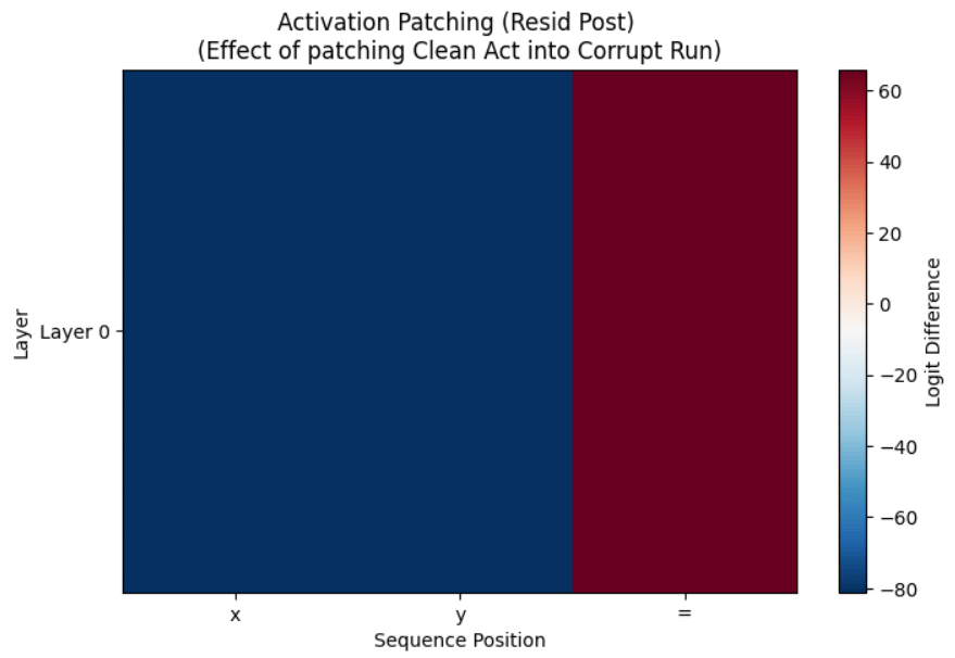
The results establish the causal link necessary to finish the puzzle.
RESULTS
By using PCA, DFT, ablation, linear probing, and activation patching, we can now confidently describe the algorithm the model uses:
The model embeds the input numbers into a 128-dimensional space where each dimension corresponds to a frequency component. The embedding for an input number is approximately [cos(k1n), sin(k1n), cos(k2n), sin(k2n), …].
At position 0, the model uses attention to gather the embedding of the first input (a). At position 1, the model gathers the embedding of the second input (b). At position 2, the model uses attention to combine these two signals.
The MLP uses the identities cos(k(a + b)) = cos(ka)cos(kb) − sin(ka)sin(kb) and sin(k(a + b)) = sin(ka)cos(kb) + cos(ka)sin(kb) and computes the products and sums, effectively rotating the inputs and combining them.
The residual stream at position 2 now encodes cos(k(x + y)) and sin(k(x + y)) for each target frequency. The unembedding matrix decodes this back to a logit (probability) over the 113 possible answers.